The SDC Process
This section presents the SDC process in a step-by-step representation and can be used as guidance for the actual SDC process. It should be noted, however, that jumping between steps and returning to previous steps is often required during the actual SDC process, as it is not necessarily a linear step-by-step process. This guidance brings together the different parts of the SDC process as discussed in the previous sections and links to these sections. The case studies in the next section follow these steps. This presentation is adapted from HDFG12. Fig. 21 at the end of this section presents the entire process in a schematic way.
Step 1: Need for confidentiality protection
Before starting the SDC process for a microdata set, the need for confidentiality protection has to be determined. This is closely linked to the interpretation of laws and regulations on this topic from the country in which the data originates and thus country-specific. A first step is to determine the statistical units in the dataset: if these are individuals, households or legal entities, such as companies, a need for disclosure control is likely. There are also examples of microdata for which there is no need for disclosure control. Examples could be data with climate and weather observations or data with houses as statistical units. Even if the primary statistical units are not natural or legal persons, however, the data can still contain confidential information on natural or legal persons. For example, a dataset with houses as primary statistical units can also contain information on the persons living in these houses and their income or a dataset on hospitalizations can include information about the hospitalized patients. In these cases, there is likely still a need for confidentiality protection. One option to solve this is to remove the information on the natural and legal persons in the datasets for release.
One dataset can also contain more than one type of statistical unit. The standard example here is a dataset containing both information on individuals and households. Another example is data with employees in enterprises. All types of statistical units present in the dataset have to be considered for the need of SDC. This is especially important in case the data has a hierarchical structure, such as individuals in households or employees in enterprises.
In addition, one has to evaluate whether the variables contained in the dataset are confidential or sensitive. Which variables are sensitive or confidential depends again on the applicable legislation and can differ substantially from country to country. In case the dataset includes sensitive or confidential variables, SDC is likely required. The set of sensitive variables and confidential variables together with the statistical units in the dataset determine the need for statistical disclosure control.
Step 2: Data preparation and exploring data characteristics
After assessing the need for statistical disclosure control, we should prepare the data and, if there are multiple, combine and consider all related data files. Then we explore the characteristics and structure in the data, which are important for the users of the data. Compiling an inventory of these characteristics is important for assessing the utility of the data after anonymization and producing an anonymized dataset, which is useful for end users.
The first step in data preparation is classifying the variables as sensitive or non-sensitive, and removing direct identifiers such as full names, passport numbers, addresses, phone numbers and GPS coordinates. In case of survey data, an inspection of the survey questionnaire is useful to classify the variables. Furthermore, it is necessary to select the variables that contain relevant information for end users and should be included in the dataset for release. At this point, it can also be useful to remove variables other than direct identifiers from the microdata set to be released. An example can be a variable with many missing values, e.g., a variable recorded only for a select group of individuals eligible for a particular survey module, and missing values for the rest. Such variables can cause a high level of disclosure risk while adding little information for end users. Examples are variables relating to education (current grade), where a missing value indicates that the individual is not currently in school, or variables relating to childbirth, where a missing value indicates that the individual has not delivered a child in the reference period. Missing values in themselves can be disclosive, especially if they indicate that the variable is not applicable. Often variables with the majority of values missing are deleted at this stage already. Other variables that might be deleted at this stage are those too sensitive to be anonymized and released or those not important to data users and that could increase the risk of disclosure.
Relationships may exist among variables in a dataset for a variety of reasons. For instance, variables can be mutually exclusive in cases where several binary variables are used for each category. An individual not in the labor force will have a missing value for the sector in which this person is employed (or more precisely not applicable). Relationships may also exist if some variables are ratios, sums or other mathematical functions of other variables. Examples are the variable household size (as a count of individuals per household), or aggregate expenditure (as a sum of all expenditure components). A certain value in one variable may also reduce the number of possible or valid values for another variable; for example, the age of an individual attending primary education or the gender of an individual having delivered a child. These relationships are important for two reasons: 1) they can be used by intruders to reconstruct anonymized values. For example, if age is suppressed but another variable indicates that they are in school, then it is still possible to infer a likely age range for that individual. Another example is if an individual is shown to be active in Sector B of the economy. Even if the labor status of this individual is suppressed, it can be inferred that this person is employed. 2) the relationships in the original data should be maintained in the anonymized dataset and inconsistencies should be avoided (e.g., SDC methods should not create 58-year-old school boys, or married 3-year-olds), or the dataset will be invalid for analysis. Another example is the case of expenditures per category, where it is important that the sum of the categories adds up to the total. One way to guarantee this is to anonymize the totals and then recalculate the sub-categories according to the original shares of the anonymized totals.
It is also useful at this stage to consolidate variables that provide the same information where possible, so as reduce the number of variables, reduce the likelihood of inconsistencies and minimize the variables an intruder can use to reconstruct the data. This is especially true if the microdata stems from an elaborate questionnaire and each variable represents one (sub-) question leading to a dataset with hundreds of variables. As an example, we take a survey with several labor force variables indicating whether a person is in the labor force, employed or unemployed, and if employed, in what sector. The data in Table 26 illustrates this example. It is possible that each type of sector has its own binary variable. In that case, this set of variables can be summarized in two variables: one variable indicating whether a person is in labor force and another indicating the employment status, as well as the respective sector if a person is employed. These two variables contain all information contained in the previous five variables and make the anonymization process easier. If data users are used to a certain release format where including all five variables has been the norm, then it is possible to transform the variables back after the anonymization process rather than complicating the anonymization process by trying to treat more variables than is necessary. This approach also guarantees that the relationships between the variables are preserved (e.g., no individuals will be employed in several sectors).
| Before | After | |||||
|---|---|---|---|---|---|---|
| In labor force | Employed | Sector A | Sector B | Sector C | In labor force | Employed |
| Yes | Yes | Missing | Yes | Missing | Yes | B |
| No | No | Missing | Missing | Missing | No | No |
| Yes | Yes | Yes | Missing | Missing | Yes | A |
| Yes | Yes | Missing | Yes | Missing | Yes | B |
| Yes | Yes | Missing | Missing | Yes | Yes | C |
| Yes | No | Missing | Missing | Missing | Yes | No |
Besides relationships between variables, we also gather information about the survey methodology, such as strata, sampling methods, survey design and sample weights. This information is important in later stages, when estimating the disclosure risk and choosing the SDC methods. It is important to distinguish between a full census and a sample. For a full census, it is common practice to publish only a sample, as the risk of disclosure for a full sample is too high, given that we know that everyone in the country or institution is in the data (see also the Section `Special case: census data <anon_methods.html#Special case: census data`__). Strata and sample weights can disclose information about the area or group to which an individual belongs (e.g., the weights can be linked with the geographical area or specific group in case of stratified sampling); this should be taken into account in the SDC process and checked before release of the dataset.
Step 3: Type of release
The type of release is an important factor for determining the required level of anonymization as well as the requirements end users have for the data (e.g., researchers need more detail than students for whom a teaching file might be sufficient) and should be clarified before the start of the anonymization process. Data release or dissemination by statistical agencies and data producers is often guided by the applicable law and dissemination strategies of the statistical agency, which specify the type of data that should be disseminated as well as the fashion.
Generally, there exist three types of data release methods for different target groups (the Section Release types provides more information on different release types):
- PUF: The data is directly available to anyone interested, e.g., on the website of the statistical agency
- SUF: The data is available to accredited researchers, who have to file their research proposals beforehand and have to sign a contract; this is also known as licensed file or microdata under contract
- Available in a controlled research data center: only on-site access to data on special computers; this is also known as data enclave
There are other data access possibilities besides these, such as teaching files or files for other specific purposes. Obviously, the required level of protection depends on the type of release: a PUF file must be protected to a greater extent than a SUF file, which in turn has to be protected more than a file which is available only in an on-site facility, since the options the intruder can use the data are limited in the latter case.
Besides the applicable legislation, the choice of the type of release depends on the type of the data and the content.
Note
Not every microdata set is suitable for release in any release type, even after SDC.
Some data cannot be protected sufficiently – it might always contain information that is too sensitive to be published as SUF or PUF. In such cases, the data can be released in on-site facilities, or the number of variables can be reduced by removing problematic variables.
Generally, the release of two or more anonymized datasets, e.g., tailored for different end users from the same original, is problematic because it can lead to disclosure if the two were later obtained and merged by the same user. The information contained in one dataset that is not contained in the other can lead to unintended disclosure. An exception is the simultaneous release and anonymization of a microdata set as PUF and SUF files. In this case, the PUF file is constructed from the SUF file by further anonymization. In that way, all information in the PUF file is also contained in the SUF file and the PUF file does not provide any additional information for users that have access to the SUF file.
Note
The anonymization process is an iterative process where steps can be revisited, whereas the publication of an anonymized dataset is a one-shot process.
Once the anonymized data is published, it is not possible to revoke and publish another dataset of the same microdata file. This would in fact mean publishing more than one anonymized file from the same microdata set, since some users might have saved the previous file.
Step 4: Intruder scenarios and choice of key variables
After determining the release type of the data, the possibilities of how an individual in the microdata could (realistically) be identified by an intruder under that release type should be examined. For PUF and SUF release the focus is on the use of external datasets from various source. These possibilities are described in disclosure or intruder scenarios, which specify what data an intruder could possibly have access to and how this auxiliary data can be used for identity disclosure. This leads to the specification of quasi-identifiers, which are a set of variables that are available both in the dataset to be released and in auxiliary datasets and need protection.
Note
If the number of quasi-identifiers is high, it is recommended to reduce the set of quasi-identifiers by removing some variables from the dataset for release.
This is especially true for PUF releases. Disclosure scenarios can also help define the required level of anonymization.
Drafting disclosure scenarios requires the support of subject matter specialists, assuming the subject specialist is not the same as the person doing the anonymization. Auxiliary datasets may contain information on the identity of the individuals and allow identity disclosure. Examples of such auxiliary data files are population registers and electoral rolls, as well as data collected by specialized firms.
Note
External datasets can come from many sources (e.g., other institutions, private companies) and it is sometimes difficult to make a full list of external data sources.
In addition, not all external data sources are in the public domain. Nevertheless, proprietary data can be used by the owner to re-identify individuals and should be taken into account in the SDC process, even if the exact content is not known. Also, the variables or datasets may not coincide perfectly (e.g., different definitions, more or less detailed variables, different survey period). Nevertheless, they should be considered in the SDC process.
Disclosure scenarios include both identity and inferential disclosure. The disclosure depends on the type of release, i.e., different data users have different data available and may use the data in a different way for re-identification. For example, a user in a research data center cannot match with large external datasets as (s)he is not permitted to take these into the data center. A user of a SUF is bound by an agreement specifying the use of the data and consequences if the agreement is breached (see the Section Release types ). Furthermore, it should be evaluated whether, in case of a sample, possible intruders have knowledge as to which individuals are in the sample. This can be the case if it is known which schools were visited by the survey team, for example. A few examples of disclosure scenarios are (see the Section Disclosure scenarios for more information):
- Matching: The intruder uses auxiliary data, e.g., data on region, marital status and age from a population register, and matches them to released microdata. Individuals from the two datasets that match and are unique are successfully identified. This principle is used as an assumption in several disclosure risk measures, such as \(k\)-anonymity, individual and global risk, as described in the Section Measuring Risk. This scenario can apply to both PUFs and SUFs.
- Spontaneous recognition: This scenario should be considered for SUF files, but is especially important for data available in research data centers where outliers are present in the data and data is often not strongly anonymized. The researcher might (unintentionally) recognize some individuals he knows (e.g., his colleagues, neighbors, family members, public figures, famous persons or large companies), while inspecting the data. This is especially true for rare combinations of values, such as outliers or unlikely combinations.
Step 5: Data key uses and selection of utility measures
In this step, we analyze the main uses of the data by the end users of the released microdata file. The data should be useful for the type of statistical analysis for which the data was collected and for which it is mostly used. The uses and requirements of data users will be different for different release types. Contacting data users directly or searching for scientific studies and papers that use similar data can be useful when collecting this information and making this assessment. Alternatively, this information can be collected from research proposals by researchers when applying for microdata access (SUF) or user groups can be set up. Furthermore, it is important to understand what level of precision the data users need and what types of categories are used. For instance, in the case of global recoding of age in years, one could recode age in groups of 10 years, e.g., 0 – 9, 10 – 19, 20 – 29, … Many indicators relating to the labor market use categories that span the range 15 – 65, however. Therefore, constructing categories that coincide with the categories used for the indicators keeps the data much more useful while at the same time reducing the risk of disclosure in a similar way. This knowledge is important for the selection of useful utility measures, which in turn are used for selecting appropriate SDC methods.
The uses of the data depend on the release type, too. Researchers using SUF files require a higher level of detail in the data than PUF users.
Note
Anonymization will always lead to information loss and a PUF file will have reduced utility. If certain users require a high level of detail, release types other than PUF should be considered, such as SUF or release through a research data center.
In the case of SUFs, it is easier to find the main uses of the data since access is documented. One way to obtain information on the use of PUF files is to ask for a short description of intended use of the data before supplying the data. This is, however, useful only if microdata has been released previously.
Statistics computed from the anonymized and released microdata file should produce analytical results that agree or almost agree with previously published statistics from the original data. If, for instance, a previously published primary school enrollment rate was computed from these data and published, the released anonymized dataset should produce a very similar result to the officially published result. At the very least, the result should fall within the confidence region of the published result. It might be the case that not all published statistics can be generated from the published data. If this is the case, a choice should be made on which indicators and statistics to focus, and inform the users as to which ones have been selected and why.
As discussed in the Section Measuring Utility and Information Loss, it is necessary to compute general utility measures that compare the raw and anonymized data, taking into consideration the end user’s need for their analysis. In some cases the utility measures can give contradicting results, for example, a certain SDC method might lead to lower information loss for labor force figures but greater information loss for ratios relating to education. In such cases, the data uses might need to be ranked in order of importance and it should be clearly documented for the user that the prioritization of certain metrics over others means that certain metrics are no longer valid. This may be necessary, as it is not possible to release multiple files for different users. This problem occurs especially in multi-purpose studies. For more details on utility measures, refer to the Section Measuring Utility and Information Loss.
Note on Steps 6 to 10
The following Steps 6 through 10 should be repeated if the data has quasi-identifiers that are on different hierarchical levels, e.g., individual and household. In that case, variables on the higher hierarchical level should be anonymized first, and then merged with the lower-level untreated variables. Subsequently, the merged dataset should be anonymized. This approach guarantees consistency in the treated data. If we neglect this procedure, the values of variables measured on the higher hierarchical level could be treated differently for observations of the same unit. For instance, the variable “region” is the same for all household members. If the value ‘rural’ would be suppressed for two members but not for the remaining three, this would lead to unintended disclosure; with the household ID the variable region would be easy to reconstruct for the two suppressed values. The Sections Household risk and Household structure provide more details on how to deal with data with household structure in R and sdcMicro.
Step 6: Assessing disclosure risk
The next step is to evaluate the disclosure risk of the raw data. Here it is important to distinguish between sample data and census data. In the case of census data, it is possible to directly calculate the risk measures when assuming that the dataset covers the entire population. If working with a sample, or a sample of the census (which is the more common case when releasing sample data), we can use the models discussed in the Section Measuring Risk to estimate the risk in the population. The main inputs for the risk measurement are the set of quasi-identifiers determined from the disclosure scenarios in Step 4 and the thresholds for risk calculations (e.g., the level of \(k\)-anonymity or the threshold for which an individual is considered at risk). If the data has a hierarchical structure (e.g., a household structure), the risk should be measured taking into account this structure as described the Section Household risk.
The different risk measures described in the Section Measuring Risk each have advantages and disadvantages. Generally, \(k\)-anonymity, individual risk and global risk are used to produce an idea of the disclosure risk. These values can initially be very high but can often very easily be reduced after some simple but appropriate recoding (see Step 8: Choice and application of SDC methods). The thresholds shall be determined according to the release type. Always remember, though, that when using a sample, the risk measures based on the models presented in the literature offer a worst-case risk scenario and might therefore be an exaggeration of the real risks for some cases (see the Section Individual risk).
Step 7: Assessing utility measures
To quantify the information loss due to the anonymization, we first compute the utility measures selected in Step 5 using the raw data. This creates a base for comparison of results obtained when using the anonymized data – i.e., in Step 10.
Note
If the raw data is a sample, the utility measures are an estimate with a variance and therefore it is useful to construct confidence intervals in addition to the point estimates for the utility measures.
Step 8: Choice and application of SDC methods
The choice of SDC methods depends on the need for data protection (as measured by the disclosure risk), the structure of the data and the type of variables. The influence of different methods on the characteristics of the data important for the users or the data utility should also be taken into account when selecting the SDC methods. In practice, the choice of SDC methods is partially a trial-and-error process: after applying a chosen method, disclosure risk and data utility are measured and compared to other choices of methods and parameters. The choice of methods is bound by legislation on the one hand, and a trade-off between utility and risk on the other.
The classification of methods as presented in Table 6 gives a good overview for choosing the appropriate methods. Methods should be chosen according to the type of variable – continuous or categorical – the requirements by the users and the type of release. The anonymization of datasets with both continuous and categorical variables is discussed in the Section Classification of variables.
In general for anonymization of categorical variables, it is useful to restrict the number of suppressions by first applying global recoding and/or removing variables from the microdata set. When the required number of suppressions to achieve the required level of risk is sufficiently low, the few individuals at risk can be treated by suppression. These are generally outliers. It should be noted that possibly not all variables can be released and some must be removed from the dataset (see Step 2: Data preparation and exploring data characteristics ). Recoding and minimal use of suppression ensures that already published figures from the raw data can be reproduced sufficiently well from the anonymized data. If suppression is applied without sufficient recoding, the number of suppressions can be very high and the structure of the data can change significantly. This is because suppression mainly affects combinations that are rare in the data.
If the results of recoding and suppression do not achieve the required result, especially in cases where the number of select quasi-identifiers is high, an alternative is using perturbative methods. These can be used without prior recoding of variables. These methods, however, preserve data structure only partially. The preferred method depends on the requirements of the users. We refer to the Section Anonymization Methods and especially the Section Perturbative methods for a discussion of perturbative methods implemented in sdcMicro.
Finally, the choice of SDC methods depends on the data used since the same methods produce different results on different datasets. Therefore, the comparison of results with respect to risk and utility (Steps 9 and 10) is key to the choice made. Most methods are implemented in the sdcMicro package. Nevertheless, it is sometimes useful to use custom-made solutions. A few examples are presented in the Section Anonymization Methods.
Step 9: Re-measure risk
In this step, we re-evaluate the disclosure risk with the risk measures chosen under Step 6 after applying SDC methods. Besides these risk measures, it is also important to look at individuals with high risk and/or special characteristics, combinations of values or outliers in the data. If the risk is not at an acceptable level, Steps 6 to 10 should be repeated with different methods and/or parameters.
Note
Risk measures based on frequency counts (\(k\)-anonymity, individual risk, global risk and household risk) cannot be used after applying perturbative methods since their risk estimates are not valid.
These methods are based on introducing uncertainty into the dataset and not on increasing the frequencies of keys in the data and will hence overestimate the risk.
Step 10: Re-measure utility
In this step, we re-measure the utility measures from Step 7 and compare these with the results from the raw data. Also, it is useful here to construct confidence intervals around the point estimates and compare these confidence intervals. The importance of the absolute value of a deviation can only be interpreted knowing the variance of the estimate. Besides these specific utility measures, general utility measures, as discussed in the Section Measuring Utility and Information Loss , should be evaluated. This is especially important if perturbative methods have been applied. If the data does not meet the user requirements and deviations are too large, repeat Steps 6 to 10 with different methods and/or different parameters.
Note
Anonymization will always lead to at least some information loss.
Step 11: Audit and Reporting
After anonymization, it is important to check whether all relationships in the data as identified in Step 2, such as variables that are sums of other variables or ratios, are preserved. Also, any unusual values caused by the anonymization should be detected. Examples of such anomalies are negative income or a pupil in the twentieth grade of school. This can happen after applying perturbative SDC methods. Furthermore, it is necessary to check whether previously published indicators from the raw data are reproducible from the data to be released. If this is not the case, data users might question the credibility of the anonymized dataset.
An important step in the SDC process is reporting, both internal and external. Internal reporting contains the exact description of anonymization methods used, parameters but also the risk measures before and after anonymization. This allows replication of the anonymized dataset and is important for supervisory authorities/bodies to ensure the anonymization process is sufficient to guarantee anonymity according to the applicable legislation.
External reporting informs the user that the data has been anonymized, provides information for valid analysis on the data and explains the limitations to the data as a result of the anonymization. A brief description of the methods used can be included. The release of anonymized microdata should be accompanied by the usual metadata of the survey (survey weight, strata, survey methodology) as well as information on the anonymization methods that allow researchers to do valid analysis (e.g., amount of noise added, transition matrix for PRAM).
Note
Care should be taken that this information cannot be used for re-identification (e.g., no release of random seed for PRAM).
The metadata must be updated to comply with the anonymized data. Variable descriptions or value labels might have changed as a result of the anonymization process. In addition, the information loss due to the anonymization process should be explained in detail to the users to make them aware of the limits to the validity of the data and their analyses.
Step 12: Data release
The last step in the SDC process is the actual release of the anonymized data. This step depends on the type of release chosen in Step 3. Changes to the variables made under Step 2, such a merging variables, can be undone to generate a dataset useful for users.
Recommended Reading Material on Risk Measurement
Dupriez, Olivier, and Ernie Boyko. 2010. Dissemination of Microdata Files; Principles, Procedures and Practices. IHSN Working Paper No. 005, International Household Survey Network (IHSN). http://www.ihsn.org/HOME/sites/default/files/resources/IHSN-WP005.pdf
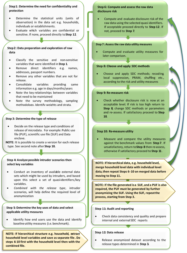
Fig. 21 Overview of the SDC process
References
| [HDFG12] | Hundepool, A., Domingo-Ferrer, J., Franconi, L., Giessing, S., Nordholt, E. S., Spicer, K., et al. (2012). Statistical Disclosure Control. Chichester, UK: John Wiley & Sons Ltd. |